MAGNET TUTORIAL

Massive Plume Migration in Northern Michigan Community

This tutorial provides step-by-step instructions for simulating one of the largest groundwater contamination plumes in the United States – and the largest TCE (trichloroethlylene) plume in Michigan. The source of the contamination is degreasing solvents used at the Wickes Manufacturing plant in the small town of Mancelona during the 1940s and ‘50s. Originally disposed into shallow pits on site, the TCE plume has migrated northwest in the surficial glacial aquifer, toward a well field providing drinking water to private properties and municipalities. TCE is a known carcinogen.

The following steps outline how use MAGNET to develop, calibrate, and apply a steady groundwater flow and transport simulator for predicting the migration of the TCE plume and simulating its removal with a groundwater purge well. Annotated graphics supplement concise written instructions. Users are encouraged to build their own model as they review the tutorial. Real-time help pages are available for the various tools/options used in the MAGNET modeling environment (see the ‘?’ buttons or the ‘Help’ sub options available throughout the menus and interfaces).

NOTE: this tutorial assumes that the reader has created a free MAGNET user account. If this has not been done, see the MAGNET Quick Helper menu in the MAGNET modeling environment (‘Help’ > ‘Quick Helper’).

1:  Create model domains (regional and local) and load/overlay the site map

Simulating the plume transport and remediation operations requires detailed information about the groundwater flow at the site. But the site-specific flow conditions are influenced by the regional flow patterns, requiring some understanding of how groundwater head is distributed in the area around (and especially upstream) of the site. The proper way to handle this ‘multiscale’ nature of groundwater systems is to simulate large-scale conditions with a larger, relatively coarse-grid model – the Regional model. This model can then be used to inform a smaller, finer grid model (the Local model).

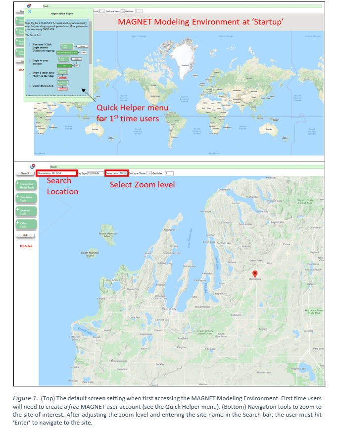
·         Use a web browser to visit the MAGNET Groundwater Modeling Environment:  https://www.magnet4water.com/magnet  (Figure 1)

·         Use the navigation tools to increase the zoom level to ‘10’ and search for Mancelona, Michigan, United States (Figure 1). Hit Enter to zoom to the general area of the site.

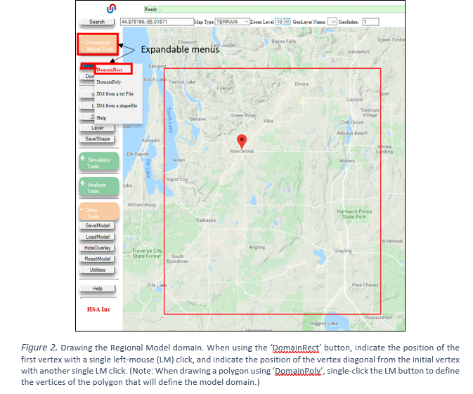
·         Use the ‘DomainRect’ tool (‘Conceptual Model’ > DrawDomain’ > ‘DomainRect’) to draw a rectangular model domain of the site and surrounding region. This will be the Regional Model domain (see Figure 2).

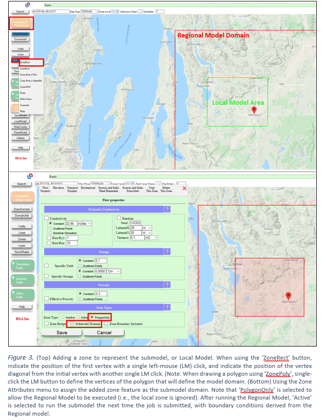
·         Use the ‘ZoneRect’ tool (‘Conceptual Model’ > ‘Zones’ > ‘ZoneRect’) to add the Local Model area, including the town of Mancelona and the area to the northwest. Click ‘SaveShape’ to finalize the shape and launch the Zone Attributes menu (Figure 3).

·         In the ‘Flow Property’ tab Zone Attributes menu, check the radio box next to ‘Submodel Domain’ and make sure the ‘PolygonOnly’ option is selected. This will be changed to ‘Active’ once the zone is needed to model the local area at and around the site (after the regional model is calibrated – see below).

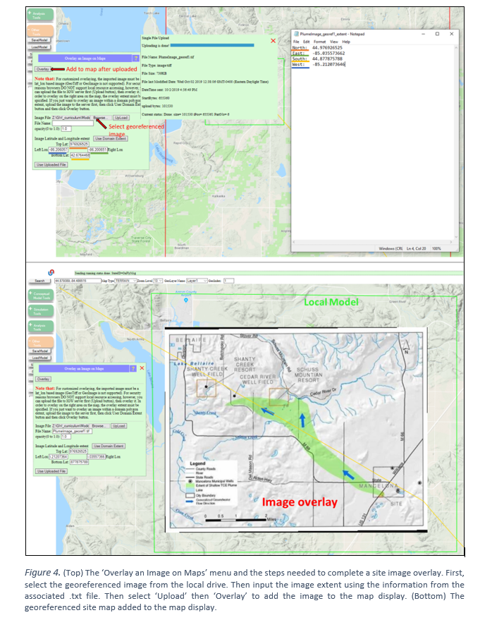
·         Use the ‘Overlay myImage’ tool to add a site map of the delineated plume to the map display (‘Other Tools’ > ‘Utilities’ > ‘Overlay myImage’)

·         Follow the instructions in the Overlay image menu (Figure 4).

o   Download and browse to the appropriate file: ‘PlumeImage_georef1’

o   Enter the image extents by copying coordinates from the following file: ‘PlumeImage_georef1_extent.txt’

o   Upload the image and coordinates to your MAGNET user account.

o   Overlay the image to the map display.

2: review/assign parameters of Regional model

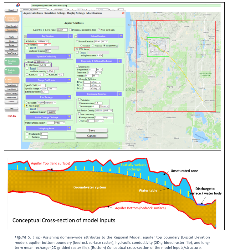
·        The model inputs/parameters are assigned using the DomainAttr (Domain Attributes) tool. This menu also provides options for numerical simulation (e.g. grid size, time-step, etc.), display settings, and projection system, among other options. (Conceptual Model Tools > ‘Domain Attr)

·        Assign the aquifer elevations – the bottom and top surfaces – by checking the appropriate radio boxes.

o    The top surface should follow the land surface characterized by the 10m Digital Elevation Model stored on the Server.

o    The bottom surface should follow the bedrock surface underlying the surficial glacial deposits. This is available as a raster layer stored on the Server.

·      The hydraulic conductivity should be input as a spatially-explicit data layer stored on the Server (‘DriftK2’ for the State of   Michigan).

·      The long-term, average recharge should be assigned as a spatially-explicit data layer stored on the Server (for the State of  Michigan).

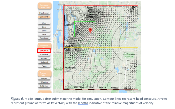
 3: simulate the Regional model and examine a cross-section

 ·         Run the model using the ‘Simulate’ tool (‘Simulation tools’ > ‘Simulate’) in steady-state mode (the default setting).

·         After confirming the projection system, the flow field will be solved.

·         Head contours and velocity vectors will be displayed in the regional model domain. Note that the number of vectors makes the display “crowded” in some areas (e.g., near the regional discharge areas).

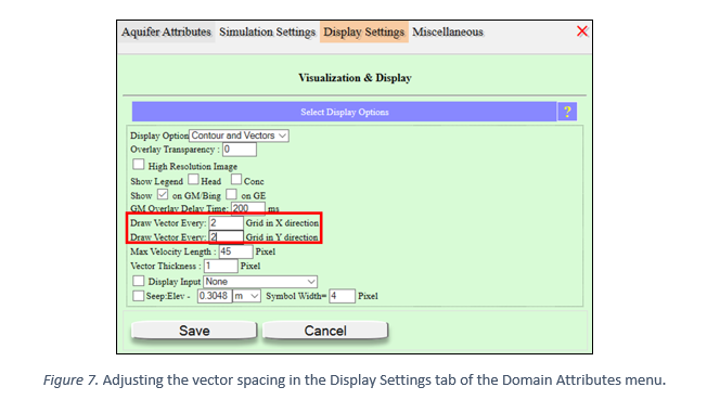
·         Reduce the vector size by navigating to the ‘Display Settings’ tab of the Domain Attributes menu and increasing the vector spacing from ‘1’ to ‘2’ pixels (see Figure 7)

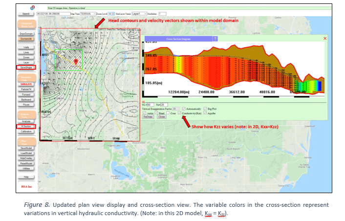
·         Use the ‘X-section’ Tool (‘Analysis Tools’ > ‘X-section’) to draw a cross-section from the regional recharge area to the regional discharge area. Click ‘ SaveShape’ (‘Conceptual Model tools’ > ‘SaveShape’) to finalize and display the cross-section in within the MAGNET modeling environment (see Figure 8). 

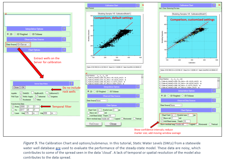
4. Evaluate model performance (calibration)

·         Compare Static Water Levels (SWLs) – measurements of water level in water wells at the time of installation (before   pumping) – to the simulated model input by using the ‘Calibration’ tool (‘Analysis Tools’ > ‘Calibration)

·         Select ‘IGWServer’ as the data source in the Calibration Chart window.

o   Filter the data to only include wells confirmed to be screen in the surficial glacial aquifer and with installation dates after 2000.

·         A comparison of simulated heads (y-axis) vs. observed heads (x-axis) will be shown in the chart display. Customize this chart:

o   Add confidence intervals of 1 standard deviation

o   Add a band-mean (moving window mean)

o   Reduce the data marker size

·         Hit ‘ReDraw’ to update the chart display. Note that the model systematically underestimates head, especially in the range of head values of 250 to 375m.

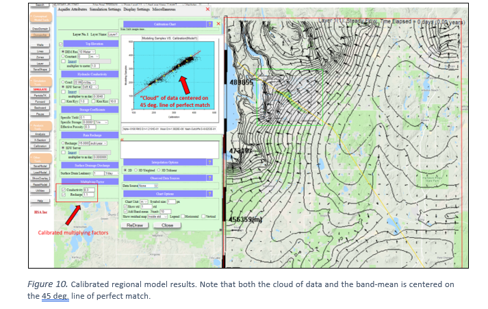
5. adjust K and recharge to improve model performance.

 ·         To improve the match between model and data, adjust model inputs within a reasonable range, e.g., hydraulic conductivity            and recharge.

·         “Multipliers” can be applied to either the hydraulic conductivity data layer or the recharge layer. For example, a hydraulic conductivity multiplier of 1.1. results in the value of each cell in the raster to be multiplied by 1.1 (or an increase of 10%).

·         Use the Domain Attributes menu to apply multipliers of 0.3 and 1.1 to the hydraulic conductivity layer and recharge layer, respectively (see Figure 10).

6. make the local model active and submit the submodel for simulation.

·         Use the results of the regional model to provide boundary conditions for the local model. Specifically, the regional model provides a spatially-variable head values along the perimeter of the local model domain. 

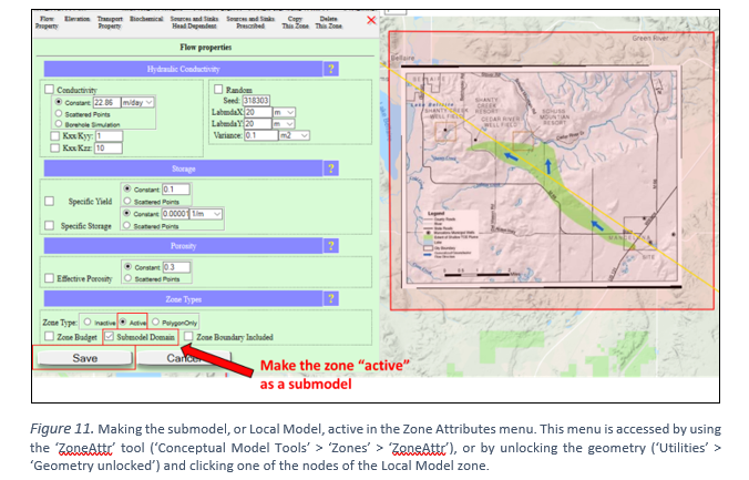
·         First, edit the local model zone.

o   Use the ‘Geometry unlocked’ tool (‘Utilities’ > ‘Geometry unlocked’) to visualize the nodes of the local model zone.

o   Click any of the nodes to launch the Zone Attributes menu.

o   Check the box next to ‘Submodel domain’ and make sure the ‘Active Option’ is selected (see Figure 11).

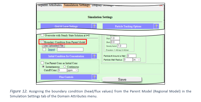
·         Then, navigate to the Simulation Settings tab of the Domain Attributes menu and check the box next to Boundary Conditions from Parent Model (see Figure 12). This utilized the last simulation result – the regional model flow field – to derive boundary conditions for the local model.

o   Note: the user can save the latest simulation results to be used as boundary conditions by selecting ‘Latest Model Zipped File’ from the ‘SaveModel’ menu. (‘Other Tools’ > ‘SaveModel’ > ‘Latest Model Zipped File’).

o   This file can then be uploaded and selected as the boundary condition for any subsequent simulation.

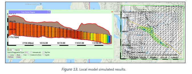
·         Submit the job for simulation and view the results. Draw a new cross-section to visualize the flow patterns along the direction of the TCE plume (see Figure 13). 

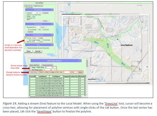
7. Adding a stream feature

·         A salient feature of the site is the Cedar River, situated north-northeast of the TCE plume and flowing roughly east to west-northwest, eventually draining into Lake Bellaire.

·         Add the Cedar River as a conceptual feature using the ‘DrawLine’ tool. (‘Conceptual Model Tools’ > ‘Lines’ > ‘DrawLine’ tool).

o   Point-and-click to add stream vertices, using the map display or site map as a guide.

o   Use ‘SaveShape’ to finalize the stream feature.

·         The Line Attributes menu will launch. Assign the Cedar River line feature as a two-way, head dependent boundary condition, allowing water to be exchanged between the stream and aquifer based on the relative difference hydraulic head (Figure 14).

o   Assign the stream stage to follow the aquifer top (DEM).

o   Assign the stream bottom elevation to be 1m below the stream stage.

o   Assign a stream leakance (hydraulic conductivity per unit thickness of the streambed) of 5 m/day.

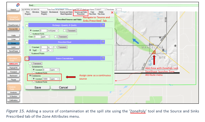
8. Add source of contamination, add a monitoring well downstream

·         Add the source of contamination at the property formely used by Wickes Manufacturing.

·         Zoom into the site (see Figure 15), then use the ‘ZonePoly’ tool to draw a zone at the site. (‘Conceptual Model Tools’ > ‘Zones’ > ‘ZonePoly’)

·         Click ‘SaveShape’ to finalize; the Zone Attributes menu will open. Navigate to the ‘Source and Sinks Prescribed’ tab, then assign the feature as a continuous source with a concentration of 1000 ppm (parts per million).

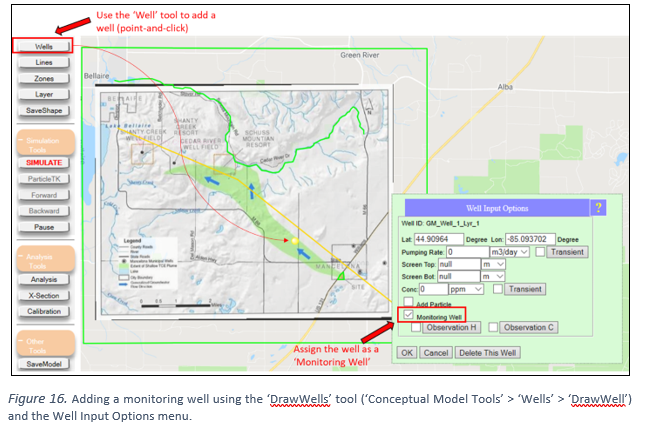
·         Use the ‘Well’ tool (‘Conceptual Model Tools’ > ‘Well) to add a monitor well downstream from the contamination site.

·         Check the box next to ‘Monitoring Well’ (see Figure 16). 

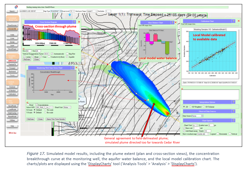
9. simulate and compare simulated transport to traditional delineation

·         Before simulating the flow and contaminant transport, assign boundary conditions from the parent model in the Domain Attributes menu (by default, ‘Boundary Conditions from Parent Model’ is unchecked after each simulation).

·         Submit local model for simulation.

·         The areal extent of the contamination and the head contours and velocity vectors will be shown in map display. The simulation is steady in the sense that the flow field does not change with time, but the plume is allowed to spread with time based on the simulated steady flow field.

·         Use the ‘DisplayCharts’ tool to show the monitoring well, cross-section view and mass balance chart in the MAGNET modeling environment ( ‘Analysis Tools’ > ‘Analysis’ > ‘Display Charts’). See Figure 17.

·         Check the model performance with the ‘Calibration’ tool.

Note that the local model performs reasonably well: there is a good match in the calibration chart; and the plume direction and extent is generally consistent with the plume delineated with traditional hydrogeological field methods.

You may also notice that the simulated plume is not “pulled” to the west as field data/site map suggests in does in reality. This is because the model does not simulate the Cedar River well field near Shanty Creek Resort. Wells can be added to the model using the ‘DrawWell’ tool (‘Conceptual Model Tools’ > ‘Wells’ > ‘DrawWell’) – see Figure 16. 

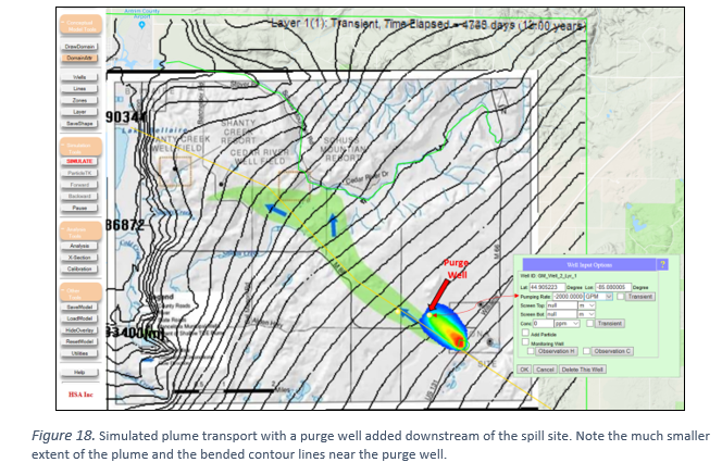
10. Add purge wells to remove contamination

·         Add a purge well to the model to remove the contaminated groundwater from the surficial aquifer.

·         Use the ‘DrawWell’ tool to add an extraction well downstream from the source of contamination.

o   Assign an aggressive pumping rate: 2000 GPM. (Note that it should be a negative value for pumping/extraction.)

·         Submit the model for simulation (after ensuring the boundary conditions are coming from the parent model). Visualize the plume migration now that the purge well has been added (see Figure 18). 

11. add vertical details – multiple computational layers and the source at the surface

The flow and plume transport has been simulated in two dimensions (XY) up to this point, with the assumption that the plume is perfectly mixed in the vertical direction. In reality, the contamination enters the groundwater system from above and is not evenly mixed in the vertical direction. ‘Computational layers’ will be added to resolve the head and concentration variability in the vertical directions.

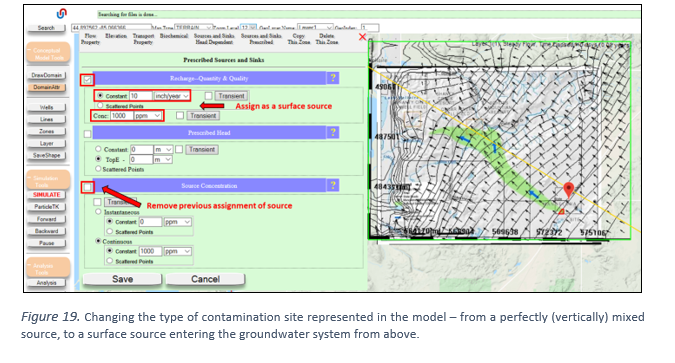
·    First convert the ‘source’ zone from a continuous source to a surface source by opening its Zone Attributes window and navigating to the ‘Source and Sink Prescribed’ tab (Figure 19).

o   Uncheck the box next to ‘Source Concentrations’.

o   Check the box next to ‘Recharge – Quantity & Quality’.

o   Enter a constant rate of infiltration (recharge) of ‘10’ inch/year.

o   Enter a source concentration (‘Conc’) of 1000 ppm.

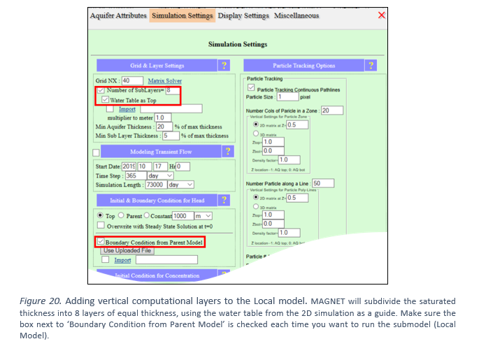
·         Sub-divide the saturated aquifer thickness into multiple (eight) vertical computational layers (Figure 20).

o   Navigate to the ‘Simulation Settings’ tab of the Domain Attributes menu.

o   Check the boxes next to ‘Water Table as Top’ and ‘Number of SubLayers’ and enter ‘8’ for the number of sublayers. This tell MAGNET to subdivide the saturated thickness into 8 layers of equal thickness, using the water table from the 2D simulation as a guide.

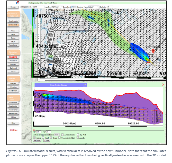
·    Double-check that the boundary conditions are derived from the Parent (Regional) model, then re-submit the model for simulation using the ‘SIMULATE’ button. Observe the plume using a cross-section (Figure 21).

Note that the simulated plume now occupies the upper ~1/3 of the aquifer rather than being vertically-mixed as was seen with the 2D model.